Right Clicking - All Options Available by Right Clicking in the GUI
Right Clicking in the Image Viewer Window
Right clicking in the main Image Viewer Window will prompt you with the following options:
‘Find Node/Edge’
Opens a text box to type the ID of a node, edge, or node community.
Entering the ID of a node/edge that is in your image will select it, highlight it, and move the image stack to its location (which requires calculating centroids in the current implementation).
In the text window, the ‘Type to Select’ dropdown menu will set whether you are searching for a node, edge, or community. (With communities being able to select multiple nodes).
‘Show Neighbors’
A neighbor is a node in a network that is one degree away from another node. Clicking ‘Show Neighbors’ reveals the following options:
- ‘Show Neighboring Nodes’
If you have any nodes or edges selected, choosing this will select and add their node-type network neighbors to the highlight display.
- ‘Show Neighboring Nodes and Edges’
If you have any nodes or edges selected, choosing this will select and add both their node-type and edge-type network neighbors to the highlight display.
- ‘Show Neighboring Edges’
If you have any edges selected, choosing this will select and add edge-type network neighbors to the highlight display.
These functions will only work correctly if the image data in the Nodes and Edges channels corresponds with that in the bottom right network table. Note that ‘edge’ neighbors means the edge object that is joining two nodes.
‘Show Connected Components’
Sometimes your network may consist of multiple, independent/unconnected components. Clicking ‘Show Connected Components’ reveals the following options:
- ‘Just Nodes’
If you have any nodes or edges selected, choosing this will select and add all node-type elements in the same connected component to the highlight display.
- ‘Nodes + Edges’
If you have any nodes or edges selected, choosing this will select and add both all node-type and all edge-type elements in the same connected component to the highlight display.
- ‘Just Edges’
If you have any nodes or edges selected, choosing this will select and add all edge-type elements in the same connected component to the highlight display.
These functions will only work correctly if the image data in the Nodes and Edges channels corresponds with that in the bottom right network table.
‘Show Community’
NetTracer3D has options to algorithmically group network nodes into communities. Clicking ‘Show Community’ reveals the following options:
- ‘Just Nodes’
If you have any nodes or edges selected, choosing this will select and add all node-type elements in the same community to the highlight display.
- ‘Nodes + Edges’
If you have any nodes or edges selected, choosing this will select and add both all node-type and all edge-type elements in the same community to the highlight display.
These functions will only work correctly if the image data in the Nodes and Edges channels corresponds with that in the bottom right network table, and the network has been community partitioned (ie, ‘Analyze -> Network -> Community Partition’)
‘Show Identity’
NetTracer3D supports the grouping of nodes into seperate ‘identities’, allowing them to represent different things. Assuming you have assigned identities, clicking ‘Show Identity’ reveals options for each identity. Clicking any of those options will select all nodes of that identity-type and add them to the highlight display.
These functions will only work correctly if the image data in the Nodes channel corresponds to the correct IDs in the ‘node_identities’ property.
You can select ‘Custom’ from this menu also to open a new window that will allow you to combine groups of identities as either positive (selects only nodes that have all those identities) or negative (does not select nodes that have said identity). This can be used to find specific combinations for multi-identity nodes.
‘Select All’
Clicking ‘Select All’ reveals the following options:
- ‘Nodes’
Selects and adds all nodes to the highlight display.
- ‘Nodes + Edges’
Selects and adds all nodes and edges to the highlight display.
- ‘Edges’
Selects and adds all edges to the highlight display.
- ‘Node in Network’
Selects and adds all nodes participating in the current network property to the highlight display.
- ‘Nodes + Edges in Network’
Selects and adds all nodes and edges participating in the current network property to the highlight display.
- ‘Edges in Network’
Selects and adds all edges participating in the current network property to the highlight display.
‘Selection’
Clicking ‘Selection’ reveals the following options. (Note this option only appears if you have a selection):
- ‘Combine Object Labels’
If multiple nodes (or edges) are selected, this option will merge those objects into a single object, and update the network property/table.
- ‘Split non-Touching Labels’
For all nodes (or edges) that are selected, this option will split any labeled objects that are not touching in space into distinct objects.
Note that this option will not automatically update the corresponding network, as it is hard to track what parts of the new objects go where in the network, so please run this before computing the network.
This current implementation of this method may be slow on larger images when many nodes are selected.
Note that running this method may likely disrupt the network labels for nodes and require the network to be recomputed, so it is better as a pre-caclulation tool.
- ‘Delete Selection’
Removes any selected nodes (or edges) from both the image and the corresponding network property/table.
- ‘Link Nodes’
If any nodes are selected, they will be assigned as new network pairs.
- ‘Split Nodes’
If any nodes are selected (and are already network pairs), their status as network pairs will be removed from the network.
- ‘Override Channel with Selection’
This option will take the region in the current highlighted display, cut said region out of a desired channel, and superimpose it onto a new channel.
The superimposed data will be transposed as to not overlap with any currently labeled regions in the new channel.
This will only superimpose the highlighted area - the rest remains the same.
Essentially, this feature can be used to take portions of one image/segmentation and incorperate them into another.
- Note that if the highlighted region is designated to be moved to an empty channel, instead an empty array will be assigned there which will absorb the ‘cut-out’ region instead.
Which can be useful to just move regions of interest to their own image.
Choosing this option will prompt the user with the following menu:
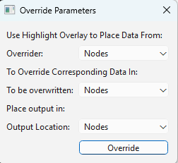
The first carrot is the channel we want the highlight overlay to extract from. Note this only provides options for the Nodes/Edges channels, as they are the only ones that can have data selected, although the options below use any channel.
The second carrot is the channel we want the highlight overlay to superimpose its extracted data onto.
The last carrot is the channel where we want the new output to be placed.
‘Measurements’
This feature can be used to extract linear or angular measurements anywhere in your dataset, both voxel-based and scaled based on the xy and z scales set by user. Clicking ‘Measurements’ reveals the following options:
- Distance - Use this menu to measure distances, revealing these options:
‘Place First Point’ (OR; ‘Place Second Point’)
This option places a measurement point at the current mouse location. If one has been placed, ‘Place Second Point’ can then be used to create a measurement.
- Angle - Use this menu to measure angles from three points, revealing these options
‘Place First Point (A)’ (OR; ‘Place Second Point (B)’ OR; ‘PLACE Third Point (C)’)
This option places points at the current mouse location. All three must be placed to measure an angle. Point ‘B’ will always be the vertex and the measured angle will always prefer the acute output.
- ‘Remove All Measurements*
This option removes all measurement points in the active session.
Data from the measurement points will be displayed in the tabulated data widget on the top right.
‘Add Highlight in Network Selection’
If any nodes or edges are selected, this method will isolate them and all their interacting neighbors into a network subgraph and place that into the ‘Selection’ table in the bottom right network widget (This is just an area that isolates data about portions of networks).
Right Clicking in the Network Table Widget
The Network Table Widget is on the bottom right of the GUI and displays information about the network. Its first two columns show linked nodes. Its third column shows if there is an associated edge object (or, 0, if there isn’t one). It has a main network table showing the full network and shown when the ‘Network’ button is enabled, and a selection window showing isolated subgraphs when the ‘Selection’ button is enabled.
‘Ctrl + F’ keyboard shortcut
All table widgets support ‘ctrl + F’ searching. In the typing window that appears, enter in a desired term and press enter to find it in the table. Press enter again to swap through all instances of that term in the tables.
Right clicking in the Main Network Table reveals the following options:
‘Sort’
Selecting sort will give the user the option to sort the network table from either low-to-high or high-to-low, using the desired column as a reference.
‘Find’
Selecting ‘Find reveals the following options’:
- Find Node/Edge:
If the mouse was over a node when right-clicking, they will be navigated to the corresponding node (assuming it exists) in the Image Viewer Window, which will be highlighted and selected.
If the mouse was over a edge when right-clicking, they will be navigated to the corresponding edge (assuming it exists) in the Image Viewer Window, which will be highlighted and selected.
- Find Pair:
Navigates the user to the corresponding pair of nodes (assuming they exist) in the Image Viewer Window. They, alongside the associated edge object (assuming it exists), will be highlighted and selected.
‘Save As’
Selecting ‘Save As provides the following options’:
- CSV
Saves the network as a .csv for analysis in generic spreadsheet software.
- Excel
Saves the network as a .xlsx for analysis in Microsoft Excel.
- Gephi
Saves the network as a .gexf file for analysis in the network analysis program ‘Gephi’
- GraphML
Saves the network as a .graphml file for analysis in a variety of different network analysis programs.
- Pajek
Saves the network as a .net file for analysis in the network analysis program ‘Pajek’.
- Pickle
Saves the network into two .pkl files. The first one contains a NetworkX Graph object corresponding to your current network, the second, some lists describing the same network. If your network is particularly big and taking a while to load in from previous sessions, you can put these pickle files in your active session folder, and it will prioritize loading them over the .CSV that it normally uses. Loading this way is slightly faster.
Right Clicking in the Selection Window
The selection window has all the same right-click options, except they will reference the selected subgraph instead of the main network. The only exception is the following option:
- Swap with network table:
Selecting this option in the selection table will cause it to be swapped with the main network table. Note that doing this will alter the internal properties of what NetTracer3D’s active session considers to be the main network.
In addition, any steps that result in a new network selection will override the ‘previous main network’ that had been swapped to the selection (as the table only stores one reference at a time).
As a result, it is advised to save any main network data that one wishes to keep before doing this.
(But use this method if you want to do more in depth analysis on a selection).
Right Clicking in the Tabbed Data Widget
The tabbed data widget stores multiple tables at once. Right clicking will always reference the one that is currently visible.
‘Ctrl + F’ keyboard shortcut
All table widgets support ‘ctrl + F’ searching. In the typing window that appears, enter in a desired term and press enter to find it in the table. Press enter again to swap through all instances of that term in the tables.
‘Sort’
Selecting sort will give the user the option to sort the table from either low-to-high or high-to-low, using the desired column as a reference.
‘Save As’
Selecting ‘Save As provides the following options’:
- CSV
Saves the table as a .csv for analysis in generic spreadsheet software.
- Excel
Saves the table as a .xlsx for analysis in Microsoft Excel.
‘Use to Threshold Nodes’
If a table is of the structure {col 1 - Integers : col 2 - Numbers}, it can be used to try to threshold what is in the nodes channel (mainly, if this table was generated in reference to said nodes). This can be used to interactively sort out any set of data that was used to analyze the nodes.
‘Close All’
Shuts all active tables (Sometimes a bunch can get populated here from doing random things, so it’s nice to clear out sometimes).
Next Steps
This concludes the explanations of the right click functions. Next, proceed to All File Menu Options for information on the file menu functions.